A superdiffusive invariance principle by iterative quantitative homogenization

We have just uploaded our paper, joint with Ahmed Bou-Rabee and Tuomo Kuusi, titled “Superdiffusive central limit theorem for a Brownian particle in a critically-correlated incompressible random drift,” to the arXiv. The results in this paper were recently announced by Ahmed in several public talks, including this one at the Fields Institute.

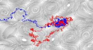
The paper is about the long-time behavior of a Brownian particle advected by a random, incompressible vector field. We consider the solution $\{ X_t \}$ of the stochastic differential equation

(1) $\begin{equation*} dX_t = \mathbf{f} (X_t) \,dt + \sqrt{2\nu} dW_t \end{equation*}$

where $\nu>0$ is a small parameter called the molecular diffusivity and $\mathbf{f}:\mathbb{R}^d \to \mathbb{R}^d$ is a stationary random vector field assumed to be divergence-free, isotropic in law, and have “critical” correlations. The model example covered by our assumptions is the case in two dimensions in which $\mathbf{f} = \nabla^\perp G$ , where $G$ is a Gaussian free field.

The general setup of (1) is classical. Since the vector field is incompressible, there are no sources or sinks and therefore we expect diffusion to be enhanced by the advection. If the vector field $\mathbf{f}(x)$ has correlations which have sufficiently fast decay, the process $X_t$ behaves diffusively for large times. Indeed, one can prove a scaling limit to a Brownian motion with covariance matrix $\sqrt{2 \overline{\mathbf{a}}}$ , for some effective diffusion matrix $\overline{\mathbf{a}}$ which is larger than $\nu I_d$ . What “sufficiently fast” means in this context, is that there exists $\xi >2$ such that

(2) $\begin{equation*} \mathrm{cov} \bigl[ \mathbf{f}(x), \mathbf{f}(y) \bigr] \simeq |x-y|^{-\xi}. \end{equation*}$

If the covariances of the vector field satisfy (2) for $\xi < 2$ , one expects to see very different, superdiffusive behavior. Here the long wavelengths of the vector field continue to cause enhancements of the diffusivity at every length scale, and if the amplitudes of these waves are large enough then they can cause the diffusivity to diverge as a function of the length scale. This case is much less well understood mathematically, due to the difficulty in analyzing the interaction of an infinite number of length scales.

This problem has been studied in the physics literature, where one can find heuristic predictions based on renormalization group arguments.

Our paper concerns the borderline case in which (2) is valid for $\xi = 2$ . In this regime, the physicists predicted (in the 1980s) a logarithmic-type superdiffusivity:

(3) $\begin{equation*} \mathbf{E}^0 \bigl[ |X_t|^2 \bigr] \simeq t \sqrt{ \log t}\,, \end{equation*}$

where $\mathbf{E}^0$ is the expectation with respect to the process starting from the origin (but not with respect to the vector field). This problem has attracted the recent attention of mathematicians (see here, here and here). These results have established (3), in the $2d$ model example described above, up to a $\nu$ -dependent prefactor and in an annealed sense—that is, after averaging simultaneously with respect to the process and the vector field $\mathbf{f}(x)$ .

Our main result: a quenched superdiffusive central limit theorem

The main result of our paper says that, almost surely with respect to the vector field, the process $X_t$ has a scaling limit to Brownian motion with a precise, superdiffusive rate.

Theorem (A. & Bou-Rabee & Kuusi 2024) There exists a constant $c_*>0$ (which in the special case of the grad-perp of the $2d$ GFF is equal to $\frac1{2\pi}$ ) such that

(4) $\begin{equation*} |\log \epsilon^2 |^{-\frac14} \epsilon X_{\frac{t}{\epsilon^2}} \Rightarrow\sqrt{2c_*} W_t\quad\mbox{as} \ \epsilon \to 0\,, \end{equation*}$

where $\{ W_t \}$ is a standard Brownian motion on $\mathbb{R}^d$ . Moreover, for every $\delta>0$ and $p\in [1,\infty)$ , there exists $C(\delta, p,d,c_*)<\infty$ such that

(5) $\begin{equation*} \mathbb{E} \biggl[ \Bigl| \frac{1}{t} \bigl[ \mathbf{E}^0[ |X_t|^2 ] \bigr] - 2d\cstar (\log t)^{\frac 12} \Bigr|^p \biggr]^{\frac1p} \leq C (\log t)^{\frac 14+\delta} \,.\end{equation*}$

Besides the scaling limit, this result:

Identifies the leading-order constant in the superdiffusivity, which in particular does not depend on $\nu.$
Goes nearly to next-order and suggests that the next term in the asymptotic expansion of $\mathbf{E}^0[ |X_t|^2 ] \bigr]$ should be of size $O( t (\log t)^{\frac 14}).$
Extends the previous rigorous results from $d=2$ to all dimensions $d\geq 2$ . In higher dimensions $d> 2$ , the typical case covered by the assumptions is when $\mathbf{f}(x)$ has a matrix potential with entries given by independent copies of the $d$ -dimensional log-correlated Gaussian field.

This result is also the first quenched one since, in contrast to the annealed results mentioned above, it proves superdiffusivity for almost every sample of the vector field. The jump from annealed estimates to quenched estimates for this problem is not a small one. Annealed estimates are often easier to obtain because one can rely on exact formulas and Gaussian identities which are available only after taking the expectation with respect to the law of the vector field. Quenched estimates, on the other hand, require completely different arguments, and I think it is fair to say that this kind of result was not completely expected, even by experts.

Heuristic derivation of the square root of log-superdiffusivity

This square root of log-superdiffusivity can be derived heuristically by thinking about the diffusivity as a function of the scale and observing how the diffusivity enhancements at each scale will give rise to a recurrence relation for these renormalized diffusivities. If $\overline{\mathbf{s}}_n$ is the renormalized diffusivity at scale $3^n$ , then this recurrence relation is roughly

(6) $\begin{equation*} \overline{\mathbf{s}}_{n+h} = \overline{\mathbf{s}}_n + \frac{c_* (\log 3) h }{\overline{\mathbf{s}}_n}\,. \end{equation*}$

The reason that $\overline{\mathbf{s}}_n$ appears in the denominator of the second term is that, as the effective diffusivity grows (as a function of the scale), the relative size of the vector field’s oscillations at these scales is smaller; consequently the enhancement due to advection is smaller.

A simple analysis of the recursion above yields that

$\begin{equation*} \lim_{n \to \infty} \frac{\overline{\mathbf{s}}_n} {\sqrt{2\cstar(\log 3)n} } = 1\,.\end{equation*}$

See Section 1.3 of our paper for a longer heuristic explanation.

The core of the proof: iterative quantitative homogenization

We start by observing that statements about the process $\{X_t\}$ can be rephrased into statements about its infinitesimal generator, which is the elliptic operator

$\mathcal{L} = \nu \Delta u + \mathbf{f} \cdot \nabla u.$

We can rewrite this as a divergence-form operator

$\mathcal{L} = \nabla \cdot \bigl( \nu I_d + \mathbf{k} \bigr)\nabla u,$

where $\mathbf{k}$ is the stream matrix for $\mathbf{f}$ , the anti-symmetric matrix (defined up to an additive constant) whose row divergence is equal to $\mathbf{f}$ .

The invariance principle is then equivalent to a statement concerning homogenization for this elliptic operator.

However, this is outside the purview of classical homogenization theory as the elliptic operator we want to analyze is unbounded. Here I do not mean simply that the coefficient matrix $\nu I_d + \mathbf{k}$ does not belong to $L^\infty$ . Far worse, its $L^2$ oscillation in a ball $B_R$ scales like $\sqrt{\log R}$ , which obviously diverges as $R\to \infty$ . Therefore, we have a large ellipticity contrast homogenization problem, with the ellipticity contrast actually getting worse as a function of the scale. The need for quantitative homogenization estimates is apparent, as one needs to homogenize the scales before the growing elliptic contrast can hurt you.

Moreover, unlike classical homogenization problems, here we need to iterate quantitative homogenization estimates an infinite number of times. This is intrinsic to the problem, since there are an infinite number of active scales responsible for the divergence of the renormalized diffusivities and thus the superdiffusivity.

In short, we need to use homogenization methods to formalize the renormalization group arguments of the physicists, and this requires new ideas and methods.

This strategy is very similar to a paper we wrote last year with Vlad Vicol. There we also used iterated, quantitative homogenization to prove anomalous diffusion for an advection-diffusion equation. The difference here is that our vector field is random and not built ad hoc from periodic ingredients. We are therefore faced with an (iterated) stochastic homogenization problem rather than a periodic one, and our active scales have no scale separation. The trade-off is that the superdiffusivity we prove here is less fast.

A detailed overview of our proof strategy appears in Section 1.4 of the paper. It is based on the “renormalization and coarse-graining” approach to quantitative homogenization we have developed in recent years, and it relies on new quantitative homogenization results for high ellipticity contrast problems (which appear in a new preprint, joint with Tuomo Kuusi, which will be posted to the arXiv very soon).

Beyond the setting of this particular problem, we hope the present paper serves as a “proof of concept” that (infinitely) iterative quantitative homogenization can be used to formalize renormalization group arguments.

yu gu

04/02/2024 at 9:50 am

I didn’t realize that the large ellipticity contrast is actually related to the correlation property of the coefficient — originally i thought it’s just that the coefficient can be close to zero and infinity. Is this stressed somewhere in the paper I can read? Thanks!

Scott Armstrong
05/18/2024 at 10:32 am

I’m sorry for the late reply Yu– I was not monitoring comments and didn’t see yours until now.

In this case, the anti-symmetric part of the coefficient field is the random field, and as you know its critical (logarithmic) correlations means that its $L^2$ oscillation in a ball $B_R$ will be of order $(\log R)^{1/2}$ . In $L^\infty$ it would be $\log R$ . Since constant anti-symmetric matrices are not seen by the equation, what really matters in any finite domain is this oscillation. Thus, it grows like $\sqrt{\log (R) }$ . But the size of the anti-symmetric matrix is related to the ellipticity. In fact, if your field is $\nu I_d + \mathbf{k}(x)$ , like we have here, then the ellipticity is actually the square of the $L^2$ oscillation of $\mathbf{k}$ divided by $\nu^2$ . So for this problem, ellipticity grows like the log of the length scale. This is why you are in a “race” between homogenization (making the effective ellipticity smaller) and the growing disorder (making it the ellipticity larger).

A superdiffusive invariance principle by iterative quantitative homogenization

2 thoughts on “A superdiffusive invariance principle by iterative quantitative homogenization”

Leave a Comment Cancel Reply